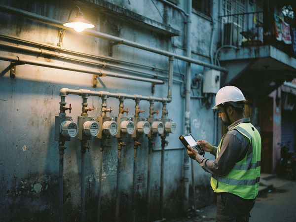
When a municipal water utility installs the first continuous monitoring points on a distribution network that has never been measured at sub-daily intervals, the initial data stream almost always contradicts the utility's own operational assumptions. The night minimum flow, which the operations team expected to be around 15 to 20 percent of the daytime average, arrives as a reading of 40 percent or higher. The pressure at the zone inlet, which the engineers assumed was stable at 4.5 bar, fluctuates between 3.2 and 5.8 bar over a single 24-hour cycle. The flow balance calculation, which the utility believed was accurate to within 5 percent, shows a gap of 18 percent on the second day of data. None of these numbers are anomalies in the monitoring system - they are the first accurate description of what the network has been doing for years, now visible at 15-minute intervals instead of monthly summaries.
The Night Minimum Flow Baseline Exceeds Every Previous Estimate
The most consistent finding across new monitoring deployments is that the night minimum flow - the lowest flow recorded between 2:00 AM and 4:00 AM when legitimate consumption should be near zero - is substantially higher than the utility's own estimates. In a typical Indian municipal network serving a population of 200,000 to 500,000, the utility may have calculated unaccounted-for water at 25 to 30 percent based on monthly bulk meter readings and consumer billing data. The first week of continuous flow data from the zone inlet meter often shows a night minimum flow equivalent to 35 to 50 percent of the average daytime flow. This is not a measurement error. It is the signature of background leakage that has been running undetected because no one was looking at the 2:00 AM data.
The operational meaning of this pattern is specific. When the night minimum flow remains flat and elevated across multiple consecutive nights, with no step changes or gradual declines, the leakage is distributed rather than concentrated. It is not a single burst that could be located by acoustic methods. It is thousands of small leaks at joints, service connections, and ferrule points that collectively consume a flow rate equivalent to a small transmission main. The utility's previous estimate of unaccounted-for water was not wrong in the aggregate - it was wrong in its distribution. The loss was assumed to be administrative or metering-related. The continuous data proves it is physical.
Pressure Data Reveals Zone Boundaries That Were Never Verified
The second pattern that emerges within the first week of monitoring is that the pressure data contradicts the zone boundary map. Most Indian municipal networks were expanded incrementally over decades, with new distribution mains tapped into existing lines without formal isolation valves or boundary meters. The utility's GIS map shows a discrete DMA boundary. The pressure data shows a zone that is hydraulically connected to an adjacent area through a valve that was left partially open or a connection that was never documented. The pressure at the monitoring point drops when a pump starts in the adjacent zone. The night minimum flow in the monitored zone increases when the adjacent zone reduces its supply hours. The two zones are not separate - they are one system operating under two different management regimes.
This has a direct operational consequence. When a utility attempts to calculate a zone-level water balance using the assumed boundary, the closing figure contains a systematic error that no amount of meter calibration can fix. The inflow meter measures water that leaves the zone into the adjacent area. The consumption data captures only the billed customers within the intended boundary. The resulting unaccounted-for water figure is inflated by a volume that is not actually lost - it is simply transferred. The continuous pressure data exposes this within 72 hours. The utility then faces a choice: install isolation valves to enforce the boundary, or redraw the zone map to match the hydraulic reality. Most choose the latter, because it is faster and does not require shutting down supply to modify the network.
Meter Reading Intervals Create Systematic Gaps in Flow Balance Calculations
The third pattern that appears in the first month of continuous monitoring is a structural mismatch between the inflow data and the consumption data that has nothing to do with leakage. The zone inflow meter logs a reading every 15 minutes. The consumer meters, in a typical Indian utility, are read once per month, and many are estimated rather than read. The billing system aggregates consumption into a monthly total that is compared against the monthly bulk meter reading. The continuous data reveals that this comparison is mathematically invalid for any period shorter than a full billing cycle, and even then it contains a systematic timing error. The bulk meter reading for a given month includes flow that occurred between the reading date and the end of the month, while the consumer billing data includes consumption that occurred in the previous month but was recorded late.
The practical result is that the monthly flow balance calculation always shows a gap that fluctuates between 8 and 20 percent, even in a network with no physical leakage at all. The gap is not real - it is an artifact of asynchronous measurement intervals. Continuous monitoring eliminates this artifact because the operator can align inflow and consumption data to the same time window. When the utility computes a flow balance using a 24-hour window that starts and ends at the same time for both inflow and consumption, the gap drops to the range of 2 to 4 percent in a well-maintained zone. The difference between 18 percent and 3 percent is not leakage reduction. It is measurement alignment. The continuous data forces the utility to distinguish between real loss and data inconsistency, which is a distinction that monthly summaries cannot make.
The First Confirmed Anomaly Is Almost Never a Burst
When operators begin reviewing continuous monitoring data for the first time, they expect the first detected anomaly to be a major pipe burst - a dramatic pressure drop followed by a flow spike. In practice, the first confirmed anomaly in a new deployment is almost always something far less dramatic and far more instructive. It is a service reservoir overflow that occurs every night between 3:00 AM and 4:30 AM, visible as a flow spike that repeats with clockwork precision. The float valve in the elevated tank has been sticking for months. The overflow pipe discharges into a storm drain. The utility has been losing 200,000 liters per night to an overflow that no one knew existed because the tank level was checked only once per day at 8:00 AM, by which time the overflow had stopped and the tank was full.
The operators initially interpret the repeating spike as a measurement glitch or a pump cycling event. It takes three to four days of pattern analysis to confirm that the spike is real, that it occurs at the same time every night, and that it corresponds to a known tank filling schedule. The utility then dispatches a crew to inspect the tank, finds the sticking float valve, and repairs it within a day. The night minimum flow drops by 12 percent. The utility has not fixed a single leak. It has fixed an operational failure that was consuming water at a rate indistinguishable from leakage in the monthly data. This is the defining characteristic of first-month monitoring findings: the most impactful discoveries are not about pipe condition. They are about operational blind spots that have been running for years because the measurement interval was too coarse to detect them.
The Transition from Periodic Checks Changes What Operations Teams Consider Normal
Before continuous monitoring, the operations team at a typical Indian municipal utility defines normal based on a small number of data points collected at irregular intervals. The morning pressure reading at the pump station. The monthly bulk meter total. The annual water audit figure. These data points create a mental model of the network that is stable, predictable, and within acceptable bounds. The first month of continuous data destroys that mental model. The team sees that pressure drops by 1.2 bar every evening when the industrial zone draws water. They see that the night minimum flow has been rising by 0.5 percent per week for the last six months. They see that the zone inlet flow spikes for 20 minutes every time a specific pump starts, indicating a check valve that is failing.
The operational consequence of this transition is that the team's definition of normal shifts from a static value to a dynamic envelope. Normal is no longer a single number like 4.0 bar. It is a range that varies by time of day, day of week, and season. The team begins to recognize that a 0.3 bar drop between 2:00 AM and 3:00 AM is normal, but a 0.3 bar drop between 6:00 AM and 7:00 AM is a potential burst. This distinction is impossible to make without continuous data. The team also begins to trust the monitoring system's alarms not because the alarms are loud, but because the baseline is known. An alarm that triggers at 3:00 AM when the flow exceeds the historical night minimum by 15 percent is credible. An alarm that triggers at 3:00 PM when the flow exceeds an arbitrary threshold is not. The first month of data provides the baseline that makes every subsequent alarm meaningful.
The first month of continuous monitoring does not solve any problems. It reveals what the problems actually are. For a utility that has been operating on monthly summaries and annual audits, this is the most valuable information it has ever received. The utility that acts on these initial findings - that investigates the night minimum flow, verifies the zone boundaries, aligns the measurement intervals, and repairs the operational failures - will reduce its unaccounted-for water by 10 to 15 percentage points within the first quarter, not because the monitoring system fixed anything, but because it showed the utility where to look. The utility that ignores the first month of data and continues operating as before will have spent money on a monitoring system that confirms what it already believed. The data itself does not change the network. The decision to act on the data does.
Talk to Olectr about a water network monitoring pilot.