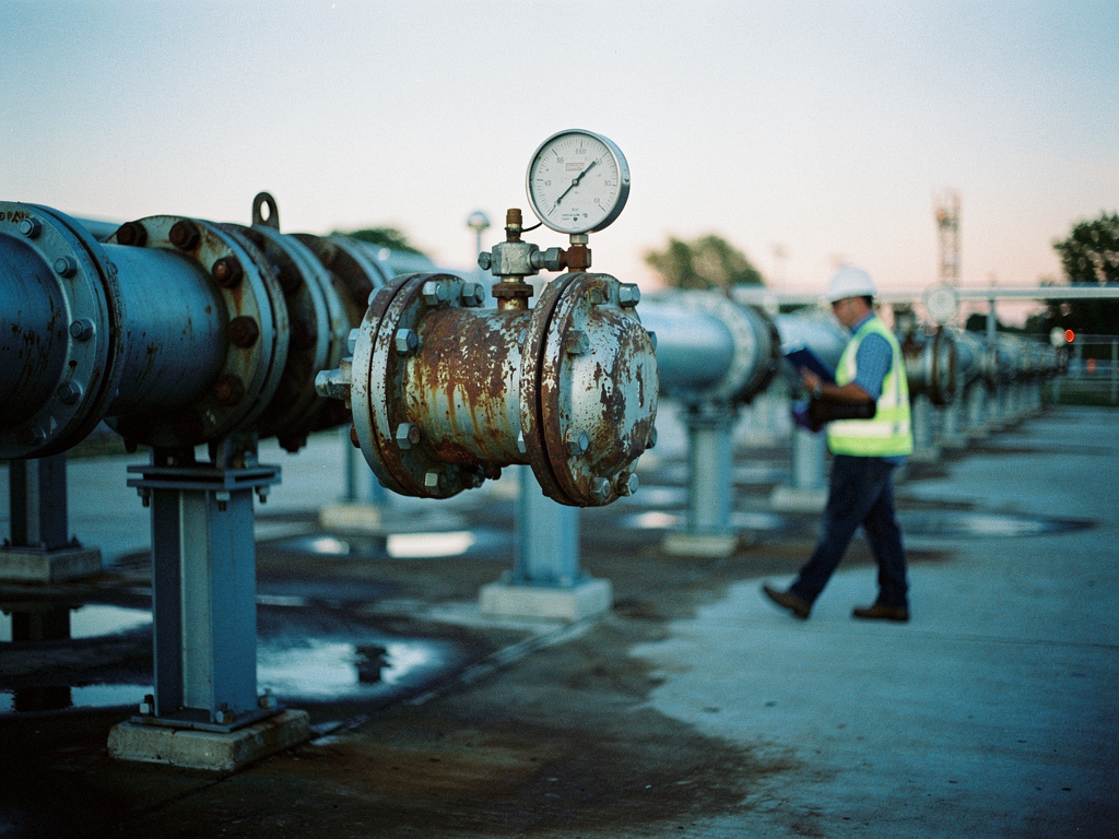
A distribution main in a municipal network does not fail suddenly. What the field crew calls a burst is the final mechanical release of a process that has been underway for weeks or months. The pipe wall loses thickness gradually. A joint seal weakens incrementally. The surrounding soil shifts under repeated loading. None of these changes are visible from the surface. But they all leave a signature in the pressure data - if the data exists at a high enough resolution and if someone is reading it correctly. Most utilities in India operate with monthly pressure readings or no readings at all. They are not missing a sudden event. They are missing a slow one that announces itself long before the water reaches the road.
Healthy Pressure Variation Follows Demand, Not Pipe Condition
A sound main in a well-operated zone shows a pressure pattern that maps directly to consumption. Night flow between midnight and 4 AM produces the highest static pressure - typically 0.2 to 0.4 bar above the daytime average in a gravity-fed system, depending on elevation and tank levels. Morning demand between 6 AM and 9 AM pulls pressure down by 0.3 to 0.6 bar as household taps open. Evening demand produces a similar dip. The pressure trace from a single sensor over a 24-hour period looks like a smooth waveform with predictable peaks and troughs. The standard deviation between consecutive 15-minute readings stays below 0.1 bar. This is the baseline that every pressure monitoring system must establish before any deterioration signal can be detected.
The critical operational fact is this: a healthy main does not show progressive pressure drift. The minimum night pressure on day 180 should be within 0.05 bar of the minimum night pressure on day 1, assuming no change in tank water level or system configuration. If the night minimum begins to drop by 0.02 bar per week over a two-month period, something has changed in the pipe or the demand pattern. The monitoring challenge is distinguishing which one.
Corrosion Thinning Produces a Distinct Pressure Drift Pattern
When internal or external corrosion reduces the wall thickness of a section of main, the pipe's stiffness decreases locally. Under operating pressure, the corroded section expands slightly more than the surrounding pipe. This micro-expansion increases the internal volume of that segment by a fraction of a percent. The measurable consequence is a gradual decline in the system's pressure response to demand changes. A 300-millimeter ductile iron main with 40 percent wall loss over a 10-meter segment will show a pressure drop during peak demand that is 0.15 to 0.25 bar greater than the same main with full wall thickness. The operator sees a pressure trace that looks like the main is serving more demand than it actually is. The flow meter at the zone inlet confirms that demand has not changed. The gap between expected pressure and measured pressure widens over weeks. This is not a leak. It is a structural weakening that will eventually become a rupture.
The pattern is identifiable because it is monotonic. Corrosion does not reverse. The pressure drift moves in one direction only - downward during demand periods - and the rate of change accelerates as the remaining wall thickness decreases. A 0.01 bar per week drift in the first three months can become 0.04 bar per week in the fourth month. The pressure trace is telling the asset manager that the failure probability is increasing, but the data must be plotted as a trend, not read as individual daily values.
Joint Failure Produces a Step Change, Not a Drift
A deteriorating joint behaves differently from a corroding pipe wall. Joints fail through gasket displacement, bolt loosening, or socket separation - each of which creates a sudden change in the mechanical boundary condition. The pressure signal from a joint failure is a step change in the night minimum pressure, typically occurring over one to three days. The operator sees a night pressure that was stable at 3.2 bar for six months drop to 3.0 bar and stay at the new level. The drop coincides with no change in tank level, valve position, or demand pattern. The flow meter may show a small increase in minimum night flow - 50 to 100 liters per minute - which points to a leak at the joint rather than a structural weakening.
The operational distinction matters because the response is different. A joint leak can often be repaired by re-tightening bolts or replacing a gasket without shutting down the main for extended periods. A corroded section requires replacement. The pressure data, when read with flow data, tells the crew which tool to bring and how long the repair will take. Without the pressure trend, the first indication of either failure mode is water on the road - by which point the asset manager has lost the opportunity to schedule the repair during low-demand hours.
A Single Pressure Sensor Cannot Separate Demand from Deterioration
This is the most common blind spot in municipal pressure monitoring. A single pressure transducer at the zone inlet records the combined effect of everything happening downstream - demand changes, valve movements, pipe deterioration, and leak development. When the pressure trace shows a gradual decline, the operator has no way to determine whether the cause is a new industrial connection drawing more water or a section of main losing structural integrity. Both produce the same downward drift in the inlet pressure reading. The only way to separate the two is to install a second pressure sensor at a critical node in the distribution network, typically at the farthest point from the inlet or at the lowest elevation point in the zone.
With two sensors, the operator can calculate the pressure differential between the inlet and the distant node under stable night flow conditions. If the differential increases over time while the inlet pressure remains constant, the added resistance is inside the pipe - either from reduced cross-sectional area due to internal scaling or from a developing leak that is drawing flow. If the differential remains constant but the inlet pressure drops, the cause is upstream - a pump issue, a tank level change, or a supply constraint. The two-sensor configuration transforms pressure data from a single ambiguous trace into a diagnostic tool that isolates the location and nature of the deterioration.
Transient Events Interact with Weakened Sections in Predictable Ways
Water hammer events - pressure surges caused by rapid valve closure or pump start-stop sequences - are routine in distribution networks. A well-maintained pipe can withstand thousands of transient events over its service life. A pipe with localized wall loss or a degraded joint cannot. The pressure data from a monitored main shows the transient amplitude at each sensor location. When a pump starts and produces a 2.0 bar surge at the inlet, the same surge may be amplified to 2.8 bar at a corroded section due to the change in wave speed through the weakened pipe wall. This amplification is measurable. The operator sees a transient spike at the downstream sensor that is consistently higher than the spike at the inlet sensor, and the amplification factor increases as the pipe condition worsens.
The practical consequence is that transient events become the trigger for failure, not the root cause. A main that fails during a pump start sequence was going to fail within weeks regardless. The transient simply accelerated the timeline. Monitoring the transient amplification over time gives the asset manager a leading indicator of failure risk. When the amplification factor at a specific sensor exceeds 1.3 for three consecutive transient events, the section between the two sensors should be inspected or replaced. The data tells the operator which segment to prioritize, not just which zone to worry about.
The 4-6 Week Window Before Failure Shows a Characteristic Signature
In the month before a confirmed pipe failure, the pressure data from a monitored main follows a consistent pattern across multiple failure types. The night minimum pressure begins to show increased variability. Instead of staying within 0.05 bar of the historical baseline, the night minimum fluctuates by 0.15 to 0.25 bar from day to day. The pressure recovery after peak demand periods slows - the trace takes 15 to 30 minutes longer to return to the static pressure level than it did three months earlier. The pressure differential between the inlet sensor and the distant node increases by 0.1 to 0.2 bar, indicating that more flow is being drawn through the deteriorating section. These signals appear together, not in isolation. Any one of them could be explained by a demand change or a valve movement. All three occurring simultaneously over a two-week period is a strong indicator that the pipe is approaching its failure point.
The operators who catch this window are the ones who review pressure trends weekly, not monthly. They compare the current week's night minimum against a rolling 30-day average. They flag any week where the night minimum drops below the 30-day average by more than 0.1 bar and the pressure recovery time exceeds the historical mean by more than 10 percent. These thresholds are not universal - they must be calibrated to each zone based on pipe material, age, and operating pressure. But the principle is consistent across networks: the failure signature is visible in the data before it is visible on the ground. The gap between the two is the asset manager's decision window.
Pressure Trend Data Changes Asset Management Decisions Fundamentally
An asset management strategy based on inspection records alone operates on a fixed schedule. The utility inspects a 500-meter section of main every five years because the pipe is 30 years old and the material is asbestos cement. The inspection finds no visible defects, so the section is not replaced. Two months later, the section fails. The inspection record was misleading because it assessed surface condition, not structural integrity. A pressure trend record, by contrast, measures the pipe's actual mechanical behavior under operating conditions. It tells the asset manager that a section with 0.15 bar of pressure drift over six months has a higher failure probability than a section of the same age with stable pressure. The replacement decision is based on measured performance, not calendar age.
This distinction has direct financial consequences. A utility that replaces mains based on pressure trend data can defer replacement on stable sections and accelerate replacement on deteriorating sections. The total replacement budget does not change, but the allocation shifts from calendar-based to condition-based. The failure rate drops because the sections that actually need replacement are the ones being replaced. The pressure data does not eliminate pipe failures - it eliminates the surprise. And in a municipal water network, the difference between a scheduled repair and an emergency burst repair is typically a factor of three to five in cost and a factor of ten in customer disruption.