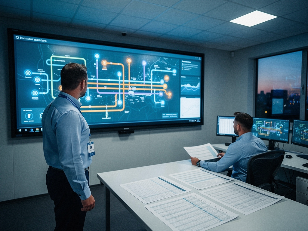
A 400-millimeter cast iron main in a central distribution zone ruptures at 3 AM. The SCADA system records a pressure drop from 4.2 bar to 1.8 bar across that DMA within eleven minutes. The night flow logger shows a sustained increase of 180 kiloliters per hour above the baseline. The GIS database, however, still shows that pipe segment as having a condition score of 7 out of 10 from an inspection conducted twenty-two months ago. That score sits in a separate database, updated quarterly, while the pressure transducer data arrives every fifteen minutes. The two datasets never meet. The engineer on the morning shift sees a pressure anomaly on the trend screen and a static pipe record in the GIS - and has no way to connect the event to the asset. That connection gap is not a technology problem. It is an operational workflow problem, and it costs utilities hours of response time every time a failure occurs.
What a GIS Layer Represents and What It Cannot Show
A municipal GIS stores pipe material, diameter, installation year, last repair date, and valve locations. These are static attributes. They describe what was installed, not what is happening to it. When a utility opens the GIS to locate a reported leak, the operator sees a line on a map with a label that reads DI 250 - 1987. That label tells the operator the pipe is ductile iron, 250 millimeters in diameter, and thirty-seven years old. It does not tell the operator whether that segment has been losing pressure for the last six nights, whether the flow into that zone has been rising gradually over the past month, or whether the adjacent valve has not been exercised since 2019.
The GIS is a record of intent and history. It is not a record of current physical condition. The moment a pipe is buried, its GIS attributes become increasingly unreliable indicators of its actual state. Corrosion progresses at rates that depend on soil resistivity, stray currents, and water chemistry - none of which appear in the asset table. A pipe that scored well in the last visual inspection can be hours away from failure if a localised corrosion cell has developed at a point where the lining has delaminated. The GIS cannot see that. Only continuous sensor data can detect the onset of that failure, and only when that data is spatially referenced to the same pipe segment does it become operationally useful.
Sensor Data Without Spatial Context Limits Operational Conclusions
A flow meter at the inlet of a DMA logs 340 cubic meters per hour at 2 AM. The minimum night flow for that zone has been 280 cubic meters per hour for the past six months. The operator sees a deviation of 60 cubic meters per hour. That number, by itself, tells the operator that something is wrong. It does not tell the operator where. The time-series graph shows the deviation started at 1:47 AM and has not returned to baseline. The operator has no way to narrow the search area without knowing which pipe segments, valves, and hydrants are downstream of that meter.
In a utility that keeps sensor data and GIS data separate, the operator must manually cross-reference the meter location against the pipe network map. This takes time. It introduces error. The operator may not know which isolation valves are operational, which segments have been replaced, or which sections are currently under repair. A 60 cubic meter per hour deviation could be a single large leak on a 300-millimeter main, or it could be a cluster of small leaks on multiple 100-millimeter laterals. Without spatial context, the operator cannot prioritize the response. The field crew is dispatched to the general zone, not to a specific street. That adds thirty to forty-five minutes to every leak response, and in a network with hundreds of leaks per year, those minutes accumulate into days of wasted crew time and thousands of kiloliters of lost water.
Associating a Fault Event with Specific Pipe Segments Changes Response Logic
When a pressure transducer logs a sudden drop and the monitoring platform automatically queries the GIS for the pipe segments within that pressure zone, the operator sees something fundamentally different. Instead of a pressure graph with a timestamp, the operator sees a list of pipe segments ranked by material, age, and repair history. The oldest unrepaired segment in the zone is a 150-millimeter asbestos cement pipe installed in 1972. The segment directly upstream of it has a recorded repair in 2018. The valve isolating that section was last exercised in 2021 and is confirmed operational. The operator now has a hypothesis: the failure is most likely on the 1972 AC segment, and the crew can be dispatched directly to that location with the valve closure sequence already determined.
This is not a futuristic capability. It is a database join between the SCADA event log and the GIS asset table, executed at the moment of detection. The join requires that the pressure zone boundaries in the GIS match the DMA boundaries in the SCADA system. That alignment is often missing in Indian municipal utilities because the GIS was built from paper records that have not been updated to reflect operational zone changes made during network modifications. When the boundaries are aligned, the response time drops from hours to minutes. The field crew arrives at the correct location, with the correct valve list, and the correct pipe material data to inform the repair method. The difference between a utility that uses GIS for record-keeping and one that uses it operationally is not the software - it is the discipline of keeping the spatial boundaries synchronised with the monitoring zones.
Spatial Analysis Reveals Patterns That Time-Series Alone Cannot Show
A time-series graph of flow into a DMA shows a gradual upward trend over six months. The operator sees the trend and suspects growing background leakage. What the time-series graph does not show is that the increase is concentrated in a cluster of three adjacent sub-zones that share a common 200-millimeter trunk main. A spatial analysis of the same data - plotting the night flow minimums for each sub-zone on a map - reveals that the three sub-zones with elevated flow are all downstream of a single valve that was partially closed during a repair eighteen months ago and never fully reopened. The flow increase is not leakage. It is a throttled valve creating a pressure differential that is pulling more water into the sub-zones than the network was designed to supply.
A utility that relies only on time-series analysis would have scheduled leak detection surveys for those sub-zones. The surveys would have found no leaks. The trend would have continued. The operator would have concluded that the leakage was diffuse and difficult to locate. The spatial analysis, performed in minutes by overlaying the flow data on the GIS pipe network, revealed the actual cause. The valve was reopened, the flow returned to baseline within twenty-four hours, and the leak detection budget was redirected to zones where it was actually needed. This pattern - a throttled valve, a closed isolation gate, a malfunctioning pressure-reducing valve - is one of the most common causes of unexplained flow increases in Indian distribution networks, and it is invisible to time-series analysis alone.
Geographic Precision Changes Field Crew Dispatch and Repair Efficiency
A utility that dispatches crews based on zone-level generalisations sends a team to a DMA boundary and tells them to start looking. The crew drives the streets, listens at hydrants, checks visible pipe runs, and may or may not find the leak within the shift. If the leak is on a branch line behind a compound wall or under a paved surface, the crew may not find it at all. The average time to locate a non-visible leak in a zone-level dispatch scenario is three to five days in Indian municipal networks, depending on the complexity of the network and the availability of listening sticks or correlators.
When the same utility generates a work order with a specific pipe segment ID, a GPS coordinate, and a list of the nearest operational valves, the crew drives directly to the location. The work order includes the pipe material and diameter, so the crew brings the correct repair coupling, the correct tapping saddle, and the correct bolt kit. They do not return to the depot to fetch a part they did not bring. The repair is completed in a single visit in most cases. The difference between a three-day location effort and a single-visit repair is not crew skill - it is the quality of the spatial information provided to the crew before they leave the depot. That information comes from a monitoring platform that reads sensor events and queries the GIS in real time, not from a printed map that was last updated when the network was extended five years ago.
The Operational Difference Between Record-Keeping GIS and Live GIS
A utility that uses GIS only for record-keeping updates the asset table when a pipe is replaced, when a new connection is added, or when an annual condition assessment is completed. The GIS becomes a historical archive. It is accurate for planning and budgeting, but it is not useful for daily operations. The operator does not open the GIS during a leak event because the GIS does not contain the information needed to respond. The operator relies on institutional knowledge - the memory of the senior lineman who knows which valves actually work and which pipes have been patched multiple times. When that lineman retires, the knowledge leaves with him.
A utility that uses GIS as an operational tool keeps the asset table synchronised with the monitoring zone boundaries, the valve exercise records, and the repair history. The GIS is updated every time a valve is operated, every time a repair is completed, and every time a zone boundary changes. The operator opens the GIS during every event because the GIS contains the current state of the network, not the design state. The difference is not the software version or the budget. It is the operational discipline of treating the GIS as a live system that must be maintained as rigorously as the physical network. A monitoring platform that integrates sensor data with GIS layers makes that discipline possible by creating a single interface where the operator sees the event and the asset together. Without that integration, the operator works in two separate worlds, and the gap between them is where response time, water loss, and repair cost all increase.