When a textile mill in an industrial estate commissioned a new 2 MVA transformer, the design engineer calculated the maximum demand at 1,650 kVA based on connected load and diversity factors from a standard handbook. Twelve months of interval meter data from the monitoring platform showed the actual maximum demand hit 1,890 kVA on a Tuesday afternoon in April, triggered not by any single large machine starting but by three simultaneous process line restarts after a power interruption. The difference between the design assumption and the operational reality cost the facility 18 percent in demand penalty surcharges for the next six months, because the contracted demand had been set too low. The data from that single event revealed something broader: the gap between how facilities plan their energy use and how they actually consume it is larger than most energy managers realize, and that gap only becomes visible when you look at continuous interval data rather than monthly bills.
Aggregate Demand Profiles Expose Design-Phase Assumptions as Fiction
The standard approach to industrial power system design relies on diversity factors published in electrical engineering handbooks. A facility with 2,000 kW of connected motor load is assigned a diversity factor of 0.75, yielding a design demand of 1,500 kW. The monitoring data from 14 medium-scale manufacturing facilities over one year showed that actual diversity factors ranged from 0.62 to 0.91 depending on shift patterns, process scheduling, and the age of motor starters. The facilities that ran continuous processes with staggered start sequences operated closer to the higher end of that range, while batch-process facilities with simultaneous machine starts regularly exceeded their design demand during transition periods between batches.
The most revealing pattern emerged during the first hour of the morning shift. In 11 of the 14 facilities, the demand spike at shift start exceeded the daily peak demand recorded during production hours. This happened because operators started multiple conveyors, compressors, and process machines within a 15-minute window, creating a coincident load that the design-phase diversity factor never accounted for. The monitoring data showed that these start-up peaks lasted between 8 and 22 minutes, long enough to register in the 15-minute demand interval used for utility billing. Facilities that had been paying demand charges based on their production-hour peaks were unknowingly being billed for these start-up transients instead.
Night-Shift and Weekend Consumption Exceeds Self-Reported Audit Figures by a Wide Margin
Energy audit reports submitted by facilities typically report night-shift consumption as a percentage of total consumption, with figures between 12 and 18 percent being common. The monitoring data told a different story. Across the 14 facilities, actual night-shift consumption averaged 31 percent of total daily consumption, with three facilities exceeding 40 percent. The discrepancy did not come from production activity - most night shifts operated at reduced capacity or handled only essential processes. The excess consumption came from support loads that audits routinely underestimate: compressed air systems leaking through unmaintained distribution networks, cooling tower fans running at full speed regardless of ambient temperature, and lighting circuits that remained energised across entire factory floors even when only a single bay was occupied.
Weekend consumption showed an even larger gap. Facilities self-reported weekend consumption at 5 to 8 percent of weekly totals. The monitoring data showed weekend consumption averaging 17 percent, with one food processing facility drawing 23 percent of its weekly energy on Saturdays and Sundays. The cause was not production - these facilities did not operate on weekends. The consumption came from HVAC systems left running in office areas, boiler pilot burners that remained lit, and battery charging stations that drew continuous current for forklifts parked over the weekend. None of these loads were metered at the sub-circuit level in any of the facilities, so they had never been visible to the energy managers who signed off on the audit reports.
Production Volume and Energy Consumption Correlate Weakly in Most Facilities
The conventional assumption in industrial energy management is that energy consumption scales with production volume. If output drops by 20 percent, energy consumption should drop by a similar margin. The monitoring data showed that this correlation held only in three of the 14 facilities, and those three were the ones with the highest proportion of direct process loads - electric furnaces, electrolysis cells, and direct-drive machinery. In the remaining 11 facilities, the correlation coefficient between daily production volume and daily energy consumption ranged from 0.34 to 0.61, meaning that production changes explained less than 40 percent of the variation in energy use.
The reason became clear when the data was disaggregated by load category. Fixed loads - lighting, compressed air, HVAC, office equipment - accounted for between 55 and 68 percent of total energy consumption in these facilities. These loads did not respond to production volume changes. When production dropped, the fixed loads remained nearly constant, compressing the energy-intensity ratio. One engineering workshop reduced its output by 35 percent over a three-month period due to a supply chain disruption, but its monthly energy consumption dropped by only 11 percent. The energy manager had been tracking energy per unit of production as a performance metric and assumed the facility was becoming less efficient. In reality, the fixed-load base was masking the performance of the variable process loads, and the monitoring data was the only way to separate the two.
Motor Load Variability Exceeds Nameplate Ratings and Reveals Operational Drift
Nameplate ratings on induction motors suggest a fixed operating point: 30 kW, 1,450 rpm, 89 percent efficiency at full load. The monitoring data showed that motors in actual service rarely operated at their nameplate ratings. Across 186 motors monitored at the 14 facilities, the average loading was 63 percent of rated capacity, with a standard deviation of 22 percent. More importantly, individual motor loads varied significantly over time. A 75 kW cooling tower fan motor at a chemical plant drew between 38 kW and 71 kW over a 24-hour period, depending on ambient temperature, fan speed settings, and the condition of the drive belt. The energy manager had been treating that motor as a fixed load in the facility's energy model.
The variability pattern carried diagnostic information. Motors that showed a gradual upward drift in current draw over weeks or months were typically experiencing mechanical degradation - bearing wear, misalignment, or pump impeller fouling. Motors that showed sudden step changes in load corresponded to process changes: a valve opened further, a conveyor belt tensioned, a damper repositioned. The monitoring data allowed operators to distinguish between these two categories, something that monthly energy bills or occasional handheld meter readings could not do. In one facility, a 45 kW pump motor showed a 12 percent increase in average current draw over six weeks. The maintenance team found a partially blocked strainer that had been gradually restricting flow and forcing the pump to operate further back on its curve. The energy cost of that undetected blockage was approximately 4,200 kWh per month, visible only in the interval data.
Maintenance Frequency and Energy Consumption Show a Direct Relationship That Facilities Do Not Track
Most facilities schedule maintenance based on running hours or calendar intervals. The monitoring data revealed that energy consumption could serve as a leading indicator for maintenance needs. In facilities where compressed air systems were serviced quarterly, the specific power consumption - kilowatt-hours per cubic meter of compressed air - increased by an average of 8 percent between service intervals. The increase was driven by pressure drops across clogged filters, increased friction in lubricated components, and higher leakage rates as seals deteriorated. The energy data showed this degradation pattern three to four weeks before the scheduled maintenance date, meaning the maintenance was being performed after the energy waste had already occurred.
The relationship was even clearer for cooling systems. Chiller plants that received maintenance on a fixed quarterly schedule showed a 14 percent increase in kilowatt-hours per ton of refrigeration between service visits. The increase was not linear - it accelerated in the final two weeks before maintenance, as condenser fouling and refrigerant charge loss compounded. Facilities that shifted to condition-based maintenance triggered by energy performance thresholds reduced their chiller energy consumption by an average of 9 percent over six months. The trigger point was not a fixed date but a 6 percent increase in specific energy consumption compared to the baseline established after the previous service. The monitoring platform calculated this automatically, allowing the maintenance team to schedule service when the data indicated it was needed rather than when the calendar dictated it.
Real-Time Monitoring Visibility Changes Some Behaviors but Not Others
The introduction of real-time energy monitoring created measurable changes in operator behavior, but the changes were not uniform across all load categories. Lighting loads showed the most significant reduction. When facility managers could see live lighting consumption on dashboards, they began switching off unused areas within the first week. The average reduction in lighting energy across the 14 facilities was 22 percent within the first three months of monitoring, and the reduction held steady over the following nine months. Compressed air systems showed a similar pattern, with a 17 percent reduction in the first quarter as operators responded to visible leakage rates and adjusted pressure setpoints.
Process loads showed a different response. The monitoring data did not cause operators to change production processes or machine settings in most facilities. The energy consumption of core production equipment remained within 3 percent of pre-monitoring levels even after 12 months of visibility. The reason was operational constraint: process parameters were set by product quality requirements and production schedules, not by energy efficiency considerations. The value of monitoring for process loads lay not in driving immediate behavioral change but in establishing baselines, detecting degradation, and quantifying the energy impact of process decisions when they were made for other reasons. One facility that adjusted its drying oven temperature setpoint for a product quality issue was able to see the 8 percent increase in energy consumption within the same shift, rather than discovering it on the next monthly bill. That visibility did not prevent the adjustment - quality took priority - but it gave the energy manager data to discuss the trade-off with the production team.
The monitoring data also revealed that the most persistent energy savings came not from operator behavior but from engineering fixes that the data enabled. A facility that installed VFDs on three cooling tower fans based on monitoring data showing continuous full-speed operation achieved a 31 percent reduction in fan energy that persisted for the entire 12-month period. A facility that repaired its compressed air distribution network after the monitoring platform quantified a 38 percent leakage rate saw the leakage drop to 11 percent and stay there. These engineering interventions, triggered by data that the monthly bills could not provide, produced savings that did not require ongoing operator attention. The behavioral changes were real but bounded; the engineering changes were permanent.